Fundamental data analysis

| Module 1: Development of practical skills in physics 1.2 Practical skills assessed in the practical endorsement |
|
|---|---|
| 1.1.2 | Use of apparatus and techniques e) Use of calipers and micrometers for small distances, using digital or vernier scales f) Correctly constructing circuits from circuit diagrams using DC power supplies, cells, and a range of circuit components, including those where polarity is important g) Designing, constructing and checking circuits using DC power supplies, cells, and a range of circuit components h) Use of a signal generator and oscilloscope, including volts/division and time-base |
a) Describe and explain:
-
I) Factors affecting accuracy and uncertainty of measurements
- Accuracy refers to how close a measured value is to the true value. Uncertainty quantifies the range within which the true value is likely to fall, reflecting the reliability of the measurement.
- ⇒ Factors affecting accuracy:
- Instrument Precision:
- – The resolution or smallest measurable unit of the instrument limits the accuracy.
- Example: A ruler with 1-mm divisions can only measure to ±0.5 mm precision.
- Calibration:
- – Improperly calibrated instruments introduce systematic errors.
- Example: A mis calibrated weighing scale might consistently overestimate weight by 2 g.
- Environmental Conditions:
- – Temperature, humidity, vibrations, or electromagnetic interference can affect measurements.
- – Example: Measuring voltage with a digital multimeter in an area with electromagnetic noise can give fluctuating readings.
- Operator Skill:
- – Human errors such as parallax (reading scales from an angle) or improper use of equipment affect accuracy.
- Example: Misreading the meniscus level in a graduated cylinder.
- Sample Variability:
- Variations in the sample being measured can affect consistency.
- Example: Measuring the diameter of an irregular object with a micrometer might yield inconsistent results.
- ⇒ Factors affecting uncertainty:
- Instrumental Uncertainty:
- – Every instrument has inherent uncertainty due to its design and limitations.
- Example: A thermometer might have an uncertainty of ±0.1°C.
- Random Errors:
- – Fluctuations caused by uncontrollable factors during measurements.
- – Example: Repeated measurements of a pendulum’s period under slight air currents yield slightly different results each time.
- Measurement Technique:
- – Poor techniques (e.g., uneven pressure in a micrometer) increase uncertainty.
- Example: Applying variable force while measuring length with a Vernier caliper.
- Data Processing:
- – Calculations using measured values propagate uncertainties.
- – Example: When multiplying two measured quantities, their relative uncertainties combine.
- Number of Measurements:
- – A single measurement is less reliable than multiple readings averaged together.
-
II) The importance of recognizing the largest source of uncertainty in a measurement
- Identifying the largest source of uncertainty is critical for improving measurement accuracy and reliability.
- Efforts to reduce the dominant source of uncertainty yield the most significant improvements in the overall confidence of results.
- ⇒ Importance:
- Effective Error Reduction:
- – Focus on the largest uncertainty allows for targeted interventions.
- – Example: In timing a falling object, if the uncertainty arises primarily from human reaction time, switching to electronic sensors eliminates this major source.
- Resource Allocation:
- – Resources can be directed toward improving the most critical aspect of the process.
- – Example: In temperature measurements, if sensor calibration contributes the most uncertainty, investing in high-quality calibration reduces errors.
- Improved Data Reliability:
- – By minimizing the dominant uncertainty, the measured values become more trustworthy and reproducible.
- Accurate Reporting:
- – Correctly identifying and stating the largest source of uncertainty allows users to evaluate the measurement’s credibility.
- – Example: Reporting the uncertainty in light intensity due to fluctuations in the power supply (rather than smaller, negligible sources) provides meaningful context.
- ⇒ Examples:
- Chemical Titration:
- – Largest source of uncertainty: Judging the endpoint by eye (color change).
- Solution: Using a pH meter or automated titration improves accuracy.
- Measuring Resistance:
- – Largest source of uncertainty: Temperature affecting the resistor.
- Solution: Performing the measurement in a temperature-controlled environment.
- Distance Measurement:
- – Largest source of uncertainty: Human error in aligning a laser rangefinder.
- Solution: Use a stable tripod or automated alignment system.
- By focusing on the largest uncertainty, scientists and engineers can make systematic improvements, increasing the reliability of their measurements.
b) Make appropriate use of:
-
I) SI units and their prefixes, standard form, angles in degrees and radians
- SI Units and Prefixes:
- – The International System of Units (SI) is the standard for scientific measurement.
- Prefixes such as milli- (m,[math]10^{-3}[/math] ), micro- (μ,[math]10^{-6}[/math]), kilo- (k,[math]10^{3}[/math] ), and mega- (M, [math]10^{6}[/math]) simplify expression of quantities across magnitudes.
- Example: Instead of expressing a distance as 0.002 meters, use 2 mm ([math]2 × 10^{-3} m[/math]).
- Standard Form:
- – Scientific notation is used to clearly express very large or small numbers.
- Example: The speed of light, [math]299,792,458m/s [/math] is expressed as [math]2.9979 × 10^8 m/s[/math].
- ⇒ Angles in Degrees and Radians:
- – Angles in degrees (0) are common in everyday use, while radians (rad) are standard in physics and engineering calculations.
- – Conversion:[math]360^0 = 2π rad (or 1^0 = π/180 \text{ rad}[/math].
- – Example: A 45° angle is [math]45 × π/180 = π/4 rad[/math].
-
II) Use of terms
- Accuracy: How close a measurement is to the true or accepted value.
- – Example: If the actual mass is 50.00 g, and the measured mass is 49.98 g, the accuracy is high.
- Precision: How closely repeated measurements agree with each other.
- – Example: Measuring 49.98 g three times is precise but not necessarily accurate.
- Resolution: The smallest change in a quantity that an instrument can detect.
- – Example: A thermometer with a resolution of 0.1°C can distinguish between 25.0°C and 25.1°C.
- Sensitivity: The response of an instrument to a small change in input.
- – Example: A balance sensitive to 0.001 g can detect minute weight changes.
- Response Time: The time an instrument takes to stabilize after a change.
- – Example: A digital thermometer might have a 2-second response time to record a temperature change.
- Uncertainty: The range within which the true value is expected to lie.
- – Example: A measured length of [math]20.0 ± 0.2cm[/math] indicates an uncertainty of 0.2 cm.
- Systematic Error: A consistent, repeatable error due to flawed equipment or methods.
- – Example: A scale consistently measuring 0.5 g heavier than the true weight has a systematic error.
- Zero Error: A specific type of systematic error where an instrument doesn’t start at zero.
- – Example: A Vernier caliper reading 0.02 mm when fully closed has a zero error of 0.02 mm.
-
III) Sketching and interpreting simple plots of measured values
- ⇒ Plotting distributions:
- Sketch: A histogram or bell curve can show the distribution of measured values.
- Mean and Spread:
- – The mean is the average of the data points, providing the central tendency.
- – The spread (standard deviation) quantifies how much values deviate from the mean.
- – Outliers: Points far from the majority indicate potential measurement errors or anomalies.
- – Reason: Outliers may arise from experimental errors, environmental disturbances, or random fluctuations.
- ⇒ Example:
- Measurements of a metal rod’s length:
- – Data: [math]100.1, 100.2, 100.5, 103.0 mm[/math]
- – Mean: [math]100.8 mm[/math]
- – Spread: Outlier at [math]103.0 mm[/math]; possible error in measurement or defective sample.
-
IV) Graphical plots and use of uncertainty bars
- ⇒ Types of Graphs:
- Scatter Plots:
- – Used to visualize the relationship between two variables.
- – Example: Plotting temperature vs. resistance for a thermistor.
- Line Graphs:
- – Show trends in data over time or another variable.
- – Example: Plot of pressure vs. volume for a gas to illustrate Boyle’s Law.

- Figure 1 Line graph
- Bar Graphs:
- – Used for categorical data or discrete measurements.
- – Example: Comparing reaction rates with different catalysts.
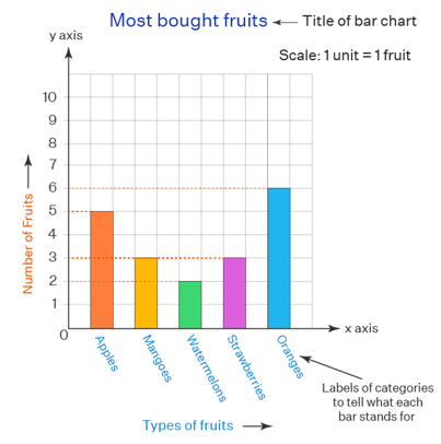
- Figure 2 Bar graph
- Uncertainty Bars:
- – Represent the range of possible values due to measurement uncertainty.
- – Example: In an experiment measuring acceleration, uncertainty bars might extend ±0.1 m/s² around each point.
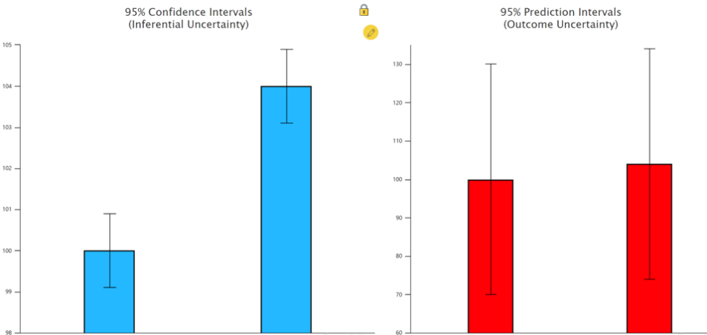
- Figure 3 Uncertainty Bars
- ⇒ Using Uncertainty Bars to Validate Data:
- If data points with uncertainty bars overlap significantly, the results are consistent with each other.
- Example: Comparing measured and theoretical values:
- – Theoretical value:
- [math]9.81 ± 0.05 m/s^2[/math]
- – Measured values:
- [math]9.78 ± 0.02 m/s^2 \text{ and } 9.83 ± 0.02 m/s^2[/math]
- – Overlapping uncertainty bars suggest that the experimental and theoretical values agree within the margin of error.
- ⇒ Identifying Errors:
- Outliers in plots with uncertainty bars may indicate systematic or random errors.
- Example: A data point with a large deviation from a linear trend might indicate incorrect calibration or an anomaly during measurement.
- This detailed approach integrates correct terminology, standard units, graphical analysis, and interpretation of uncertainty to ensure precise and reliable measurements.
-
c) Make calculations and estimates involving
-
I) Calculations involving uncertainty, mean, range, spread, and percentage uncertainties
- 1. Uncertainty of Experimental Data:
- The uncertainty of individual measurements is often given by the resolution of the instrument or calculated as the standard deviation of repeated measurements.
- – Example: Measuring the length of a rod five times:
- Measurements: [math]100.1, 100.2, 100.3, 100.2, 100.4 mm[/math]
- [math]\text{Mean} = \frac{100.1 + 100.2 + 100.3 + 100.2 + 100.4}{5} = 100.24 \text{ mm}[/math]
- Standard deviation =[math]±0.1 mm[/math].
- 2. Range and Spread:
- Range: Difference between the maximum and minimum values.
- – Example: [math] Range = 100.4 – 100.1 = 0.3 mm.[/math].
- Spread: Typically represented by the standard deviation, which shows how data points vary around the mean.
- 3. Percentage Uncertainty:
- Calculated as:
- [math]\text{Percentage Uncertainty} = \left( \frac{\text{Absolute Uncertainty}}{\text{Measured Value}} \right) \times 100[/math]
- Example: If a measurement is [math]100.2 ± 0.2 mm:[/math]:
- [math]\text{Percentage Uncertainty} = \frac{0.2}{100.2} \times 100 = 0.2\%[/math]
- 4. Best-fit Gradients and Intercepts with Uncertainty:
- To estimate the gradient of a line, use:
- [math]\text{Gradient} = \frac{\Delta y}{\Delta x}[/math]
- Uncertainty in the gradient can be determined using error bars on the data points.
- Example: If the line passes through [math](x_1, y_1) = (1.0, 2.1) [/math] and [math](x_2, y_2) = (3.0, 6.3)[/math].
[math]Gradient = (6.3-2.1)/(3.0-1.0) = 2.1.[/math]
Uncertainty in the gradient can be estimated using maximum and minimum gradients by connecting the extremes of error bars.
- Example: If the line passes through [math](x_1, y_1) = (1.0, 2.1) [/math] and [math](x_2, y_2) = (3.0, 6.3)[/math].
-
II) Estimating uncertainties in combined data
- ⇒ Rules for combining uncertainties:
- Addition/Subtraction:
- – Add absolute uncertainties:
- [math]∆z = ∆a + ∆b[/math]
- – Example:
- [math]z = a + b \text{ where } a = 5.0 ± 0.1 m \text{ and } b = 3.0 ± 0.2 m \\
z = 5.0 + 3.0 = 8.0 ± 0.3 m[/math] - Multiplication/Division:
- – Add relative (percentage) uncertainties:
- [math]\frac{\Delta z}{z} = \frac{\Delta a}{a} + \frac{\Delta b}{b}[/math]
- – Example:
- [math]z = a \cdot b \quad \text{where} \quad a = 5.0 \pm 0.1 \text{ m}, \quad b = 3.0 \pm 0.2 \text{ m} \\
\frac{\Delta z}{z} = \frac{\Delta a}{a} + \frac{\Delta b}{b} = \frac{0.1}{5.0} + \frac{0.2}{3.0} = 0.02 + 0.067 = 0.087 \\
\text{Percentage Uncertainty} = 8.7\%[/math] - Raising to Powers:
- – Multiply relative uncertainty by the power:
- [math]\frac{\Delta z}{z} = n \cdot \frac{\Delta a}{a}[/math]
- – Example:
- [math]z = a^2, \quad \text{where} \quad a = 4.0 \pm 0.1 \text{ m} \\
\frac{\Delta z}{z} = 2 \cdot \frac{0.1}{4.0} = 0.05 \\
\text{Absolute Uncertainty} = 0.05 \times (4.0)^2 = 0.8 \text{ m}^2[/math] -
III) Estimated magnitudes of everyday quantities
- Mass of a Person:
- – Estimated: 70 kg
- – Uncertainty: ±2kg (based on typical weighing scales).
- Height of a Building:
- – Estimated: 30 m (10 stories, assuming each story is approximately 3 m)
- – Uncertainty: ±1 m.
- Speed of a Car:
- – Estimated: 60 km/h on a city road
- – Uncertainty: ±5 km/h (based on typical speedometer accuracy).
- Energy Consumption of a Light Bulb:
- – Estimated: for an incandescent bulb
- – Uncertainty: ±2 W.
- Volume of a Cup of Coffee:
- – Estimated: 250 ml
- – Uncertainty: ±10 ml.
- ⇒ Example Combining Concepts
- Problem:
- A student measures the length and width of a rectangle:
- – Length:
- [math]20.0 ± 0.2 cm[/math]
- – Width:
- [math]10.0 ± 0.1 cm[/math]
- Calculate the area and its uncertainty.
- Solution:
- Calculate Area:
- [math]A = \text{Length} \times \text{Width} = 20.0 \times 10.0 = 200.0 \text{ cm}^2[/math]
- Combine Uncertainties:
- – Relative uncertainty in length:[math]\frac{0.2}{20.0} = 0.01[/math]
- – Relative uncertainty in width:[math]\frac{0.1}{10.0} = 0.01[/math]
- – Total relative uncertainty:[math] 0.01 + 0.01 = 0.2[/math]
- Absolute Uncertainty in Area:
- [math]∆A = 0.02 × 200.0 = 4.0 cm^2[/math]
- Final Result:
- [math]A = 200.0 ± 4.0 cm^2[/math]